Huge advancements in machine learning are made each year, and 2021 was not the exception. Through our consulting projects we had the chance to put some of them to work.

In this article, we share topics, techniques, and resources that had the greatest impact on our work during the year. We’ll cover transformers applied to computer vision, techniques that enhance the generation of image embeddings, and new losses to deal with the most common classification pains in the neck.

Hopefully, this article will help you navigate through these topics and apply them to your own projects. It is worth noting that it is not meant to be an exhaustive list of trends or a SoTA review. Feel free to reach out if you have any questions or comments.

Attention

tl;dr Attention-based models were introduced in NLP four years ago. Since the introduction of ViT, they have been slowly expanding to computer vision. Lately, promising work has been done around leveraging the capacity of the attention mechanisms of transformers architecture, with the generalization capabilities of convolutional blocks (CoAtNet by Google Research).

Since 2014, multiple attention strategies have been introduced to computer vision models. From channel attention, spatial attention, and temporal attention to combinations of them. With the introduction of Transformers architecture for natural language processing tasks, there have been a lot of attempts to leverage it to computer vision as well. ViT [1] was the big breakthrough for Transformers in CV. It stands for Vision Transformer and, for the first time, a model without convolutional layers was able to match state-of-the-art performance on classification datasets.

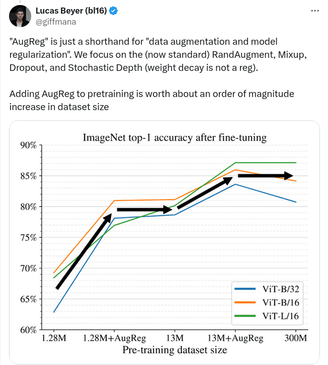
ViT created a new wave of transformer-based models in CV, which rely heavily on attention mechanisms. One of the simpler paths to getting better results is to start with a good model and scale it as much as possible. This is exactly what the authors of ViT did [2]; they leveraged the capacity of a bigger model, more training data, and AugReg (data augmentation and model regularization) techniques to make everything fit together. They released multiple models (ViT-Ti/S/B/L) with different sizes, alongside hybrid models that use a ResNet model as the backbone. Besides the new models, they provided great practical insights on how to scale transformers-based models:

• “We conclude that across a wide range of datasets, even if the downstream data of interest appears to only be weakly related to the data used for pre-training, transfer learning remains the best available option.”

• “Our analysis also suggests that among similarly performing pre-trained models, for transfer learning a model with more training data should likely be preferred over one with more data augmentation.”

One of the authors, Lucas Beyer, wrote a great Twitter thread with the main takeaways:

"AugReg" is just a shorthand for "data augmentation and model regularization". We focus on the (now standard) RandAugment, Mixup, Dropout, and Stochastic Depth (weight decay is not a reg).

Adding AugReg to pretraining is worth about an order of magnitude increase in dataset size pic.twitter.com/HbadR7eoeA

— Lucas Beyer (@giffmana) June 21, 2021

And we recommend the TIMM implementations in Pytorch: https://github.com/rwightman/pytorch-image-models

Purely transformer-based models are still behind SoTA convolutional networks. But there is a lot of opportunity in combining the two approaches. One of the models that caught our curiosity this year is CoAtNet [3] by Google Research. It leverages the model capacity of the attention mechanisms of transformers architecture, with the generalization capabilities of convolutional blocks. They were able to reach state-of-the-art performances on multiple datasets while constraining the training resources.

As concluded by Meng-Hao Guo et al. [4], attention mechanisms are key in SoTA CV models, and it is expected that there will be further progress in this direction.

References:

• An Image is Worth 16x16 Words: Transformers for Image Recognition at Scale Dosovitskiy et al., 22 Oct 2020

• How to train your ViT? Data, Augmentation, and Regularization in Vision Transformers Steiner et al., 18 Jun 2021

• CoAtNet: Marrying Convolution and Attention for All Data Sizes Dai et al., 9 Jun 2021

• Attention Mechanisms in Computer Vision: A Survey Guo et al., 15 Nov 2021

  
  

Metric learning

tl;dr Generating good embeddings is crucial. Deep metric learning leverages the capacity of deep learning models to generate them. There has been a lot of progress since the introduction of TripletLoss, such as SphereFace, CosFace, and ArcFace. The last couple of years were not the exception, new losses were introduced, as well as novel end-to-end trainable approaches (Intra-batch), and the comeback of proxy-based approaches (ProxyNCA++).

Metric learning refers to methods used to generate vector representations given a set of inputs. In computer vision, it means creating vector representations (check out our article about image embeddings) that capture semantic information from the images relevant to the task at hand. As it happens for most computer vision tasks, deep learning approaches have been dominant in metric learning. It mainly consists of choosing the right components: The feature extractor: the model architecture that will be used to map our inputs into embeddings. A distance function: a function that indicates how similar the embeddings are in the n-dimensional space. A loss: the function used to train the feature extractor.

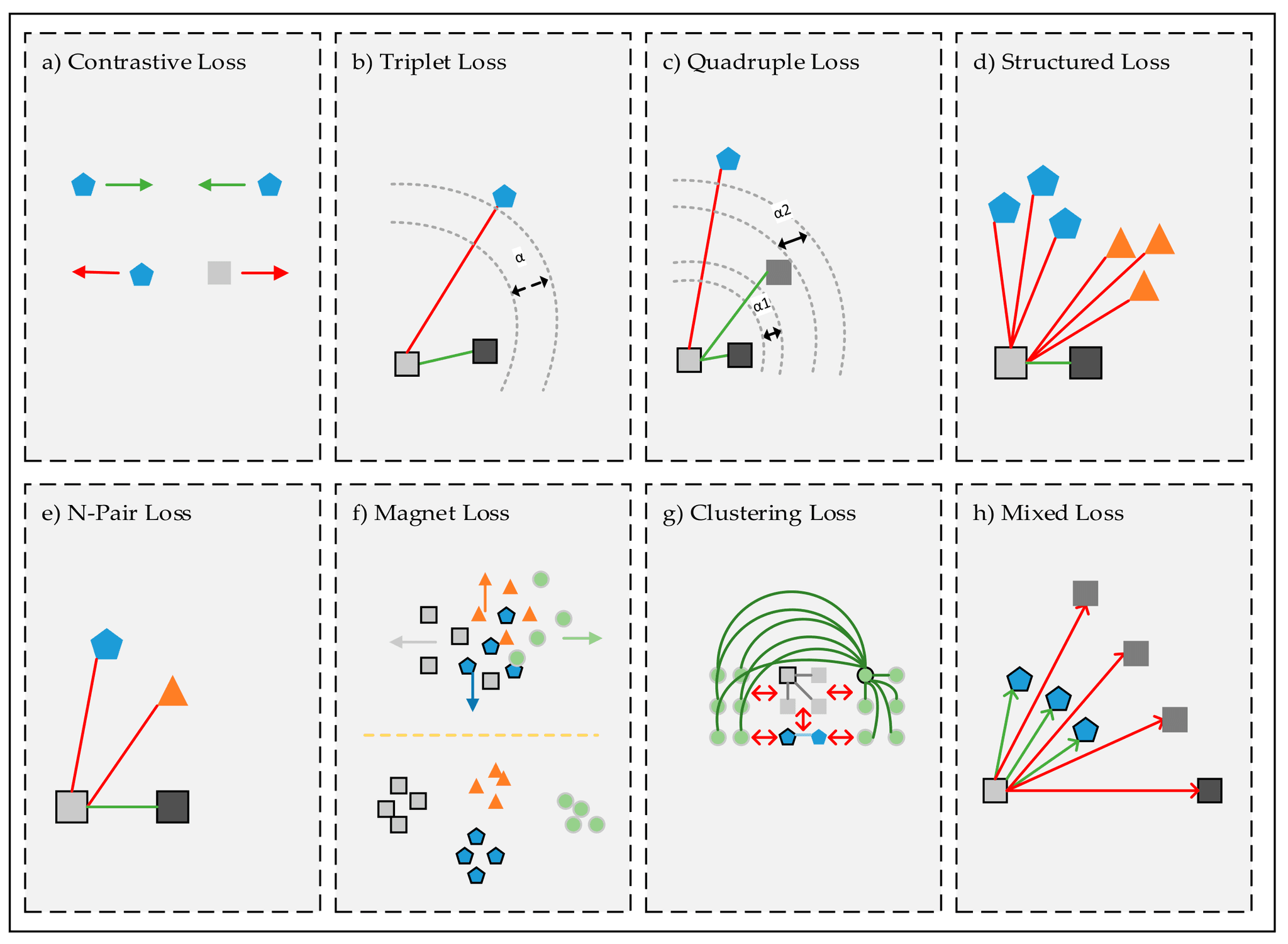
The advancements in these types of models come from newer and better losses. Since the introduction of the Triplet Loss [1], there has been a lot of progress in contrastive losses.

In 2017, the SphereFace [2] approach was introduced which relies on the angular distance and angular margins. This was followed by a new set of approaches based on this idea, including CosFace [3] and ArcFace [4]. We recommend reading the in-depth survey about deep metric learning by Chan Kha Vu.

In 2021 we had the chance to work on some challenging projects where metric learning approaches were a good fit. We started with the traditional Triplet loss and one of its extensions, the Quadruplet loss, to leverage the data available, and then we had the opportunity to explore the SoTA.

From all the advances on this area, here are the two that we highlight:

ProxyNCA++: Revisiting and Revitalizing Proxy Neighborhood Component Analysis

Teh et al, 2020

This contribution extends ProxyNCA [5] with multiple enhancements. Let’s analyze NCA and ProxyNCA before diving into ProxyNCA++.

Neighborhood Component Analysis (NCA) uses a distance metric to classify inputs into classes. Its goal “is to maximize the probability that points assigned to the same class are neighbors, which, by normalization, minimizes the probability that points in different classes are neighbors”.

ProxyNCA is inspired by NCA and it attempts to address one of NCA’s main drawbacks, NCA computational costs grow polynomially with the number of samples. ProxyNCA introduces the idea of classes proxies, embeddings that represent each class and are stored as learnable parameters. Comparing samples to proxies instead of other samples reduces the number of possible combinations.

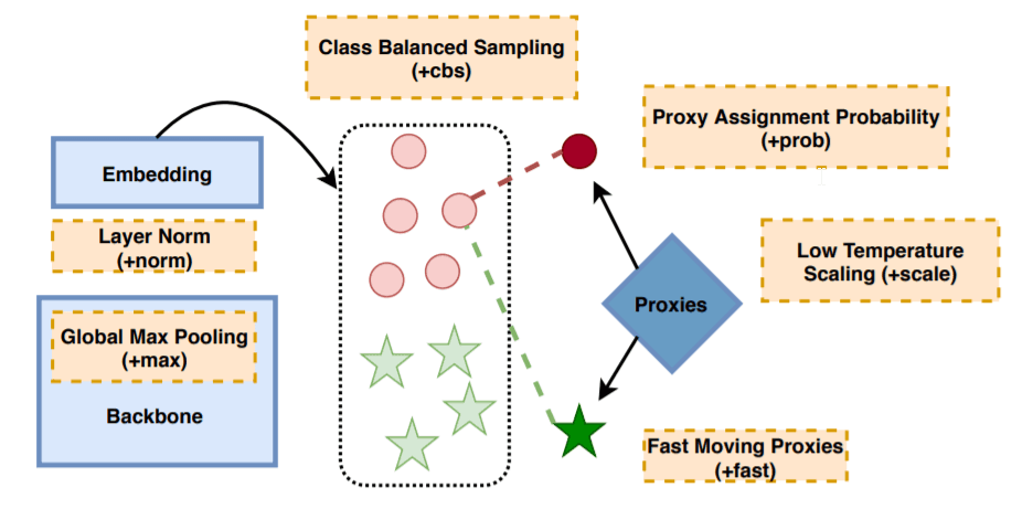
ProxyNCA++ extends the idea of ProxyNCA by applying multiple enhancements, from the way probabilities to proxies are assigned, to temperature scaling, and exploring different pooling strategies.

Official implementation at https://github.com/euwern/proxynca_pp.

Learning Intra-Batch Connections for Deep Metric Learning

Seidenschwarz et. al., 2021

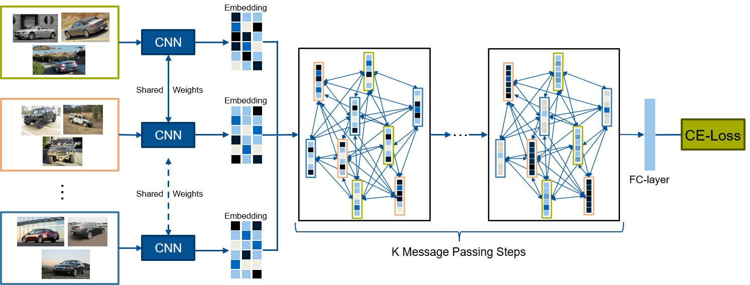
It presents a fully learnable framework that leverages MPNN [6] to exchange messages between batches in order to adjust the global distribution of the embeddings. Each node on the graph network is an embedding generated by the CNN backbone. Messages are shared between nodes of different batches to adjust the representation based on the global distribution. It also implements an attention mechanism to measure the importance of the neighbors. This allows each sample to choose what other samples to use in order to predict the decision boundary.

In comparison to the Triplet approach, this is a radical change. It removes the complexity of choosing the right triplet, and even more, it removes the triple constraints and allows samples to choose from the entire mini-batch. And as the cherry on top, the model is fully learnable and end-to-end trainable! It is an amazing contribution that has yielded SoTA results across multiple datasets.

Official implementation at https://github.com/dvl-tum/intra_batch.

References:

• FaceNet: A Unified Embedding for Face Recognition and Clustering Schroff et al., 12 Mar 2015

• SphereFace: Deep Hypersphere Embedding for Face Recognition Liu et al., 26 Apr 2017

• CosFace: Large Margin Cosine Loss for Deep Face Recognition Wang et al., 29 Jan 2018

• ArcFace: Additive Angular Margin Loss for Deep Face Recognition Deng et al., 23 Jan 2018

• No Fuss Distance Metric Learning using Proxies Movshovitz-Attias et al., 21 Mar 2017

• Neural Message Passing for Quantum Chemistry Glimer et al., 4 Apr 2017

  
  

Multilabel Classification

tl;dr Facing the challenge of a highly imbalanced dataset or a poorly tagged one is something every machine learning engineer that tackled a classification problem has encountered. In the past two years, innovative techniques and losses have been developed to solve these issues. Some of these include Asymmetric Loss, Distribution-Balanced Loss, and even estimating the labels distributions.

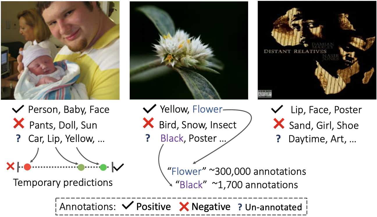
Multilabel classification is a common machine learning problem in which the goal, most of the time, is to tag an image with one or more possible tags. This presents several challenges. Firstly, there are usually a high number of possible tags, which also leads to probably under-tagged datasets. For example, in the popular dataset of OpenImages (V6), the tag “Lip” appears on 1,121 images, whereas the tag “Human Face” appears on 327,899 images. Ben-Baruch and Ridnik [1] implement a partial annotations approach to estimate the class distribution with a separate model to predict possible missed labels in the dataset to solve this issue. This method prevents the model from labeling “common” tags that are under-represented as negative during training.

The second challenge is that there is a very high-class imbalance on positive tags in most real-world cases. This manifests in long-tail distributions where positive tags are well represented, while rarer tags are widely underrepresented. Consequently, model training is a lot harder, as the model struggles to learn the rarer classes. Finally, due to the nature of this type of classification, there is a very imbalanced positive-negative relationship. The consequence is that the model ends up classifying most images as negative and makes it harder for the model to learn from the positive samples.

The consequences generated by having a highly imbalanced dataset (in the two previously mentioned ways) are worsened because most approaches for multilabel classification use Binary Cross Entropy loss (BCE), which is designed to be symmetric, so positive and negative labels are treated the same. This makes training the model even harder, as it can’t properly learn from the positive classes. To address this, Hu and Huang [2] suggest a new loss function to handle the imbalance in multi-label problems statically. They call this loss Distribution-Balanced Loss. This loss introduces a re-balanced weighting after resampling, which alleviates the impact of long-tail distributions, and negative-tolerant regularization that attempts to overcome the over-suppression of negative labels.

Further advancement of this loss was proposed by Ben-Baruch [3] called Asymmetric Loss (ASL). This loss implements two key concepts that help to address the high negative-positive imbalance and ground-truth mislabeling:

• Asymmetric Focusing

• Asymmetric Probability Shifting

We won’t go into detail in this blog post explaining these two concepts but stay tuned for our future blog post, where we will give a more technical analysis about these types of ML problems and go more in-depth in this paper. For now, this new loss function is capable of fine-tuning how much the loss is influenced by the positive and negative labels, solving the issue that most of the available labels will be negative for any given image. This way, the model learns meaningful features for the rare positive samples and generalizes a lot better, especially when the number of possible tags is big, and most labels will be negative.

Other popular methods for dealing with multi-label classification problems and long-tail distributions focus on resampling and rebalancing the dataset by eliminating images from the dataset with popular tags. This often doesn’t lead to better results as we are eliminating useful information by deleting tagged images. By changing the losses to better deal with these issues we get much better end results without any loss of information. Finally, there is a PyTorch implementation of the ASL loss that is a drop-in replacement for the classical BCE loss. The only thing to keep in mind is that this loss adds a couple of new hyperparameters that require some prior knowledge and fine-tuning.

References:

• Multi-label Classification with Partial Annotations using Class-aware Selective Loss Ben-Baruch et al., 21 Oct 2021

• Distribution-Balanced Loss for Multi-Label Classification in Long-Tailed Datasets Wu et al., 19 Jul 2020

• Asymmetric Loss For Multi-Label ClassificationBen-Baruch et al., 29 Sep 2020

  
  

Our predictions for 2022

Computer vision, as a field, advances at an impressive speed and it’s part of what draws us to the field. As a consulting company, we try to stay ahead of the curve and identify which areas (although it is very hard!) are prone to have a breakthrough in the near future. Here is a top 3 area that we believe will have the biggest impact on our solutions:

• Metric learning. Powerful architectures such as Intra-batch mentioned above will be introduced trying to leverage global information about the distributions.

• Learning from adversarial examples. Contrastive learning relies a lot on the samples chosen during training, in particular the positive. This adds complexity and restrictions to the training. Being able to artificially generate cases that reinforce positive and negative signals to the model will have huge returns.

• Learning with Limited Data. Gathering data is hard, at Pento we are constantly looking for ways to make the process cheaper. By improving the labeling process to get the most out of what is available. Of course, this is a pain to any company and luckily for us there has been a lot of progress around these types of issues.

Hope you enjoyed our main takeaways from this 2021 related to CV. Feel free to drop us a line telling us what you think and make sure to follow our blog if you’d like to read more about computer vision and what we do here at Pento. Be safe!