Object detection: An overview with code examples
Learn what object detection is and how it has evolved. Take a look at some of the most common and practical use cases. Code included.
Gonzalo Chiarlone
Engineering Manager
Learn what object detection is and how it has evolved. Take a look at some of the most common and practical use cases. Code included.
Gonzalo Chiarlone
Engineering Manager

Object detection has been a trendy topic in computer vision in the last 10 years. This shouldn't be a surprise to anybody, taking into account that it allows computers to watch the world with their own eyes (or cameras, whatever).
In this article, we will discuss object detection and how it can be used and mention some of the most popular techniques: from classic to state-of-art. Finally, we also include code examples of some of the most popular models to try yourself.
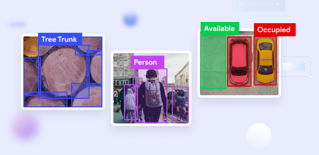
Object detection is the computer vision task that deals with the localization and, most of the time, classification of specific objects in images. This can be done by looking for a single object (left figure), multiple objects of the same class (middle figure) or even multiple objects of multiple classes (right figure).


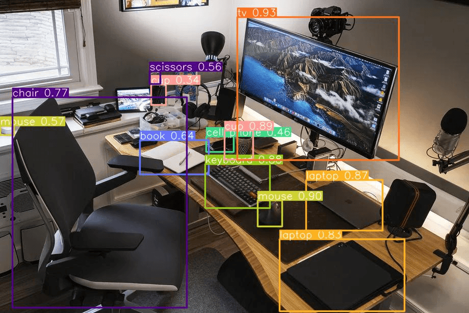
Once you familiarize yourself with the tool, it's only up to your imagination to set use cases. We will mention some of the most common ones you can find. Consider that object detection could be applied not only in a given set of images but also to a live video, applying the algorithm frame by frame.
One of the most common uses is video frame-by-frame tracking. This consists of applying an object detection algorithm to each video frame. This could be done for different purposes, like following a football player on the field, tracking a customer in a store, or ensuring nobody enters a particular zone for security purposes.
![]()
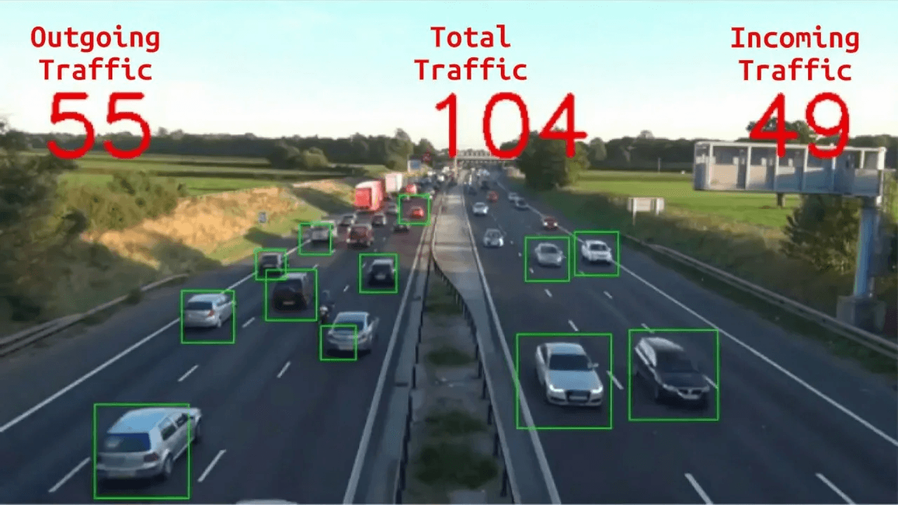
Another everyday use is counting objects in an image (or a video frame). As in many other examples, this is often faster and more reliable when done by machines rather than humans. An example of this could be counting the number of vehicles passing by like in the following figure.
Sometimes, you may want to detect objects with specific characteristics (color, size, and position). Similar to the previous example, but only looking for red cars.
Similarly, anomaly detection consists of detecting the presence of an object you don't want in an image. Sometimes we also look for the absence of the object itself. For example, you can have a camera pointing to plants and detecting if any of them is dry or has odd leaves purely based on what the camera is seeing.
Even though it is a sub-case of anomaly detection, this application has become an independent field. The idea is to detect the presence of different objects (or living beings) in a medical image (it could be a resonance, x-rays, tomography, radiography, etc.), supporting the doctors on where to look.
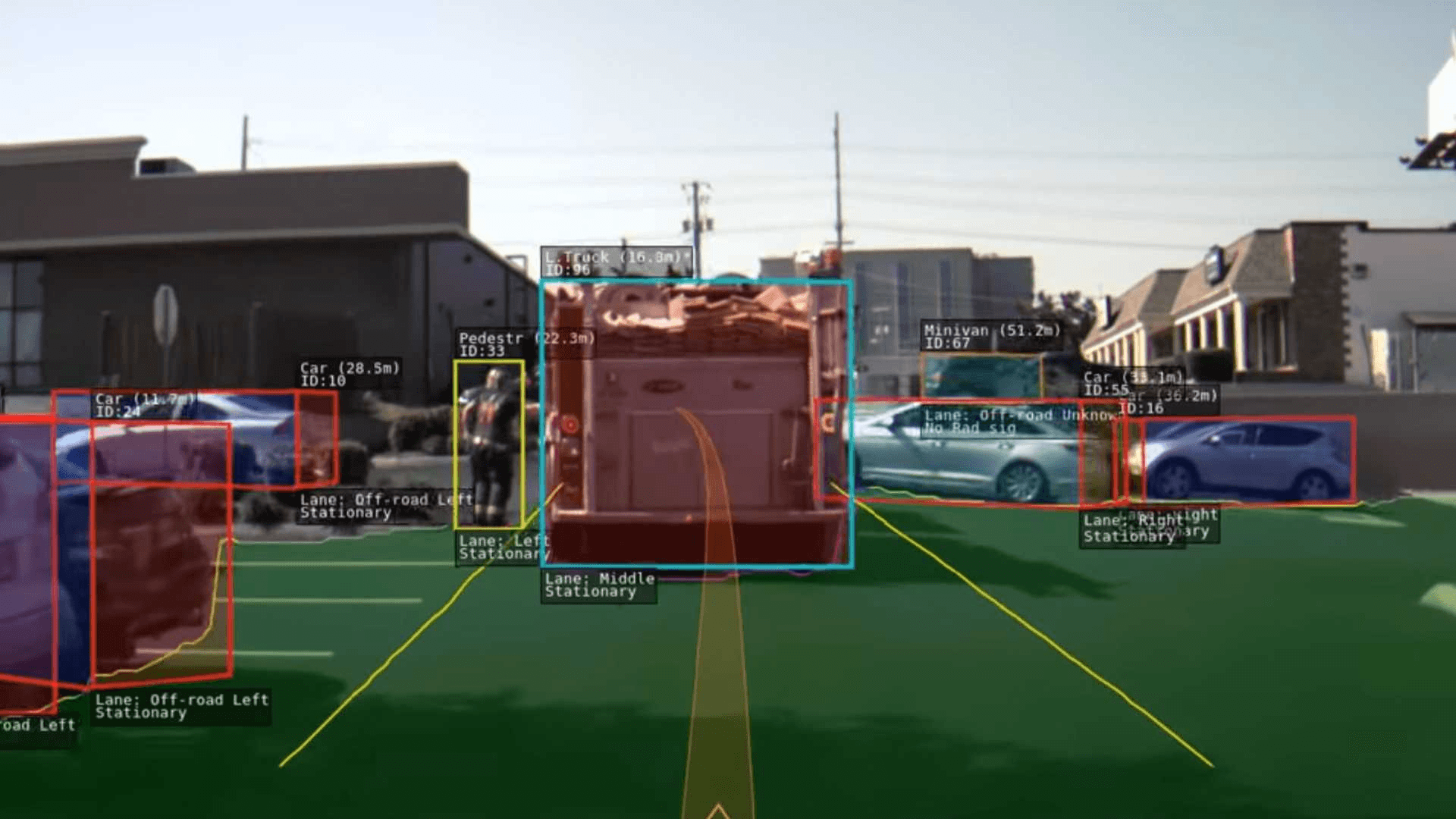
Just like all animals, robots also need to "see" the world in their own way. But sometimes, it's not enough. They have to know what they are looking at. One well-known example of this is autonomous cars, which have to distinguish between road signs, cars, pedestrians, traffic lights, etc. to decide how to respond.
Computer vision has made enormous progress in the last couple of decades, and object detection is not the exception. Just to understand on what basis it stands today, it may be helpful to see some of the most important changes in its brief history. Mainly it can be divided into two different "eras": Before and After Deep Learning (BDL and ADL).
Before using deep learning on object detection, the methods were based on hand-crafted features. These features come from various algorithms with information that can be obtained directly from the image. The methods are sometimes labeled as Traditional object detectors. There are 3 representative examples of this era:


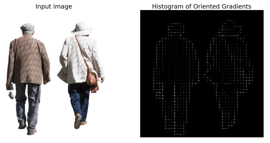
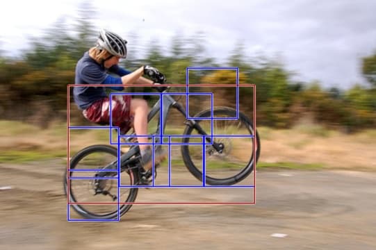
Progress got stuck around 2010 until AlexNet came up in 2012, starting the new DL era. This project implemented CNN, combined with data augmentation, and achieved the lowest error rates to that date.
CNNs had been applied to handwritten recognition, but there were computational limitations and not large enough databases to scale to object detection in a wider range of images. AlexNet tackled this problem. reference
Later on, all the different models proposed in the last decade can be sorted out into 2 main categories:
Now it's time to try a real example of object detection. For this example, we will use two well-known models: YOLOv5 (you-only-look-one) and Detic.
The first example will be using YOLOv5. This is one of the most popular algorithms nowadays and the one to go to when looking for a real-time object detector, mainly because of its incredible speed and accuracy.
Let's start by installing some dependencies:
Then, we have to load the image in which we will run the model:
If everything goes right, the following image should open:

Now we have to load the model with PyTorch:
Notice that we set the pretrained parameter True. This tells PyTorch that we want to use the weights obtained from training in the 1000-class ImageNet dataset (for more details, go to YOLOv5). These weights can be finetuned for a particular purpose if trained in a dataset of your choice (that's one of the many things we here do at Pento).
After loading the image and the model, we are now able to run the model on this image or, as we like to call it, make an inference:
If you followed every step right, probably two things should happen:
First, something like this should appear in the console:
What does this tell us? For the image in batch (1/1), with a size of 720x1280, it detected 2 objects classified as "person" and 2 classified as "ties." The rest is information about the speed of the inference.
Then, the following image should pop up:
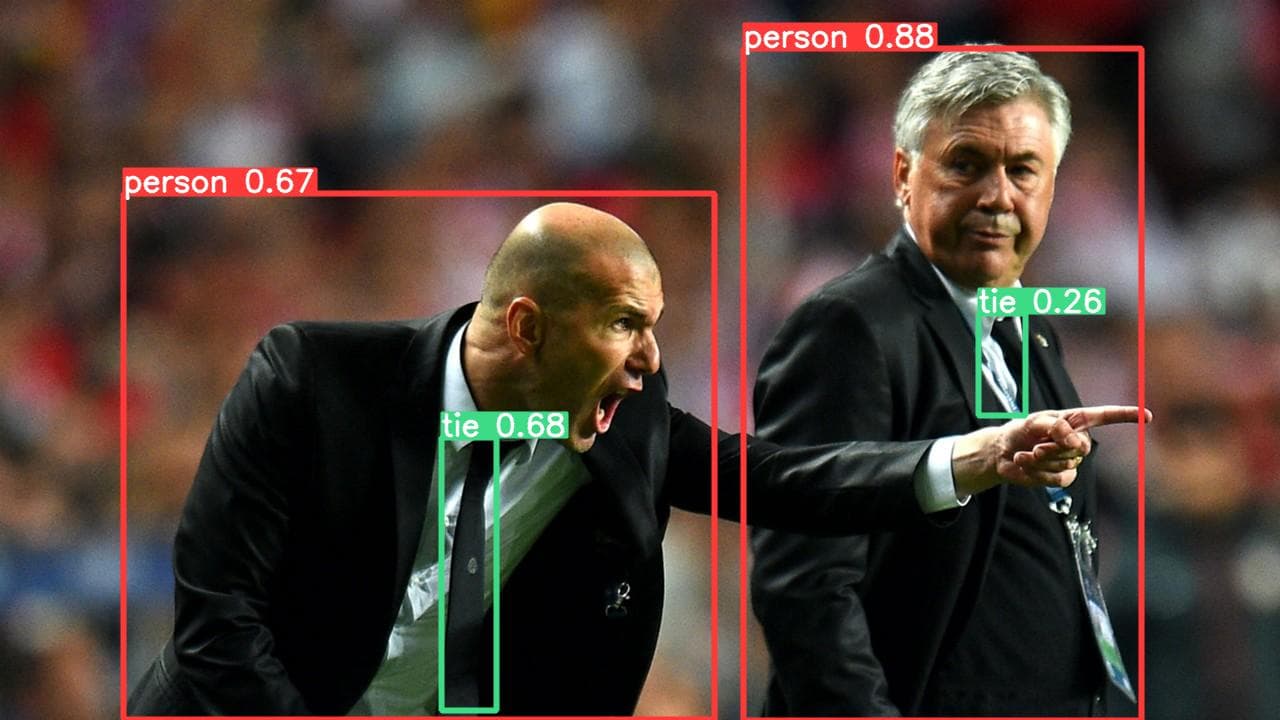
Here we can see the bounding boxes in each object, each with its respective tag and confidence the prediction is correct.
Our final example will use a newer detector called Detic (Detector with Image Classes). It can be considered a two-stage detector, which focuses on expanding the vocabulary. Primarily, it introduces Natural Language Processing to assist in the classification. But don't worry. All you need to know is that you can include more classes, resulting in images full of labels.
First, let's set up our working environment:
Now, if you only want to run Detic on a single image from the terminal, you can do it by running the following command:
However, if you want to create a programmatic file that you can run as many times as you like and customize, you can achieve it with the following code:
NOTE: This file must be inside the folder "Detic"
We start importing some dependencies and declaring some constants:
Then we have to choose the configurations of our model. Here there are two important things:
After this preparation, we can finally instance the model. We call the model "predictor" since we only make inference predictions. Notice that we have to choose a vocabulary from the ones we put in the "BUILDIN_CLASSIFIER" and "BUILDIN_METADATA_PATH." You could try changing this to obtain different results.
After that, we only need to run the model and visualize the results.
This should print us something similar to this:
And also, it should save an image named "detic_output.jpg", which should look like the image below, depending on the vocabulary you chose.
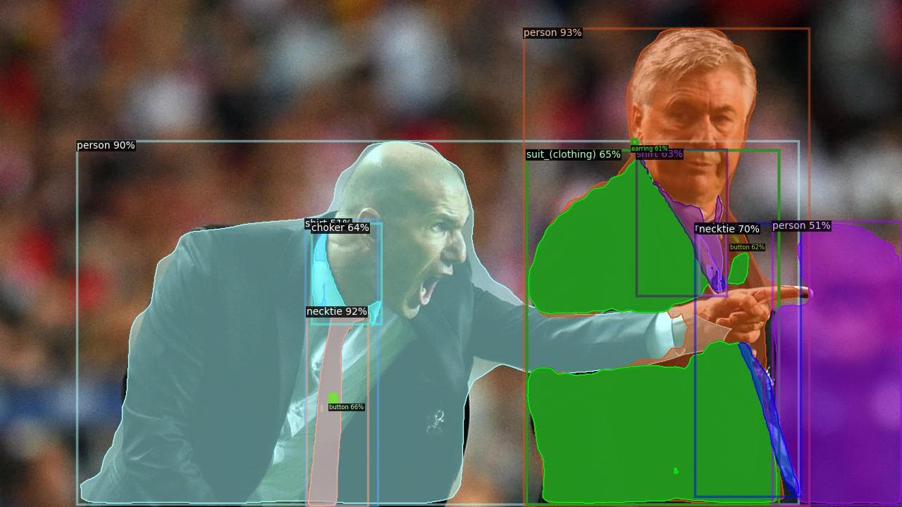
Here we can see three main differences with YOLO:
So that's it! That's all it takes to use a generic object detector! Go ahead and try it for your own set of images. Of course, a more custom solution would imply both data handling and training, but this is all you need to have your own simple object detector.
Object detection has become an essential tool for automatization in many areas, from security to medical applications. The idea here was to give you some background and two basic examples to start trying by yourself, and we hope we made it easy enough. The limit of this tool is your imagination.
You can also read

Discover the key computer vision innovations of 2022, from Latent Space Diffusion and Stable Diffusion to YOLOv7's object detection advances and cutting-edge deep metric learning techniques combining language guidance with vision models.
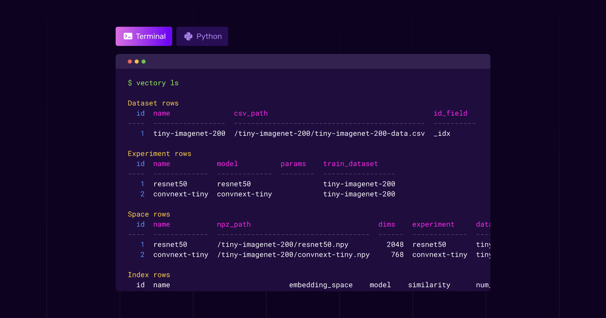
Vectory is a tool made for and by machine learning engineers who want a light and easy way to track and compare embeddings.

Super-resolution consists of using AI to automatically enhance image quality. Going from a low-resolution image to an upscaled, HD version.
CONTACT US
Work with Pento to turn promising AI experiments into systems that perform reliably in production, with the right architecture, delivery model, and engineering support.